Time Series Analysis
Time Series Analysis
Reference books:
Forecasting: Principles and Practice (3rd ed)
Topics In Mathematics With Applications In Finance
Time Series Analysis and Ist Aplications
PRINCIPLES:
- Plot the data (first)
Explore the Nature of Data (available tools)
- Graph: enable to see features; including patterns, unusual observations, changes over time, and relationships between variable.
Linear Regresion Analys
- Data set
- n cases i=1,2,...,n
- 1 response variable, yi, i=1,2,...,n
- p explanatory variables, xi =(x_(i,1), x_(i,2), ..., x_(i,p))^T, i=1,2,...,n
- Goal: extract/exploit relationship betwee yi and xi
- Examples:
- Prediction
- Causal inference
- Approximation
- Functional RElationships
Possible Models:
- Polynomial approximation
- Fourier Series
- Time series regressions
Steps for Fitting a Model [read]
- Propose a model
- specify/define a criterion for judging different estimators
- Characterize the best estimator and apply it to the given data
- Check the assumptions in (1)
- If necessary modify model and/or assumptions and go to (1)


Fit ARMA Model -
astsa
ARIMA
Forecast
Fit ARIMA model
Key Concepts:
White Noise: is a type of time series data in which the data values are uncorrelated and have constant variance. In other words, each data point is independent of the previous and next data points, and the variance of the data points is constant over time.


Which is wich?solve

Stationarity: a stable time series. Mean constant (no trend), correlation (variance and covariance) structure remains constant over time. This means that the mean and variance are constant over time, and the autocorrelation function only depends on the time lag between observations and not on the time itself. [practice]
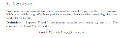
MIT-Covariance-Correlation (read the properties)


Stationary Identification:
- Plots
- Summary Statics (like mean and variance)
- Statistical tests - Unit Root Test
- Augmented Dickey-Fuller (ADF)
- Kwiatkowski-Phillips-Schmidt-Shin (KPSS)
- Phillips-Perron (PP)
These tests are similar but they have different test statistics and different critical value tables.
If the time series is not stationary, we may need to transform the data or use more complex models that can account for non-stationarity.
Transforme Data, is not stationary to get it:
- Random Walk trend in Xt- diff() - Xt-X(t-1)

Random Walk: is a stochastic process where the future value of the series is unpredictable and only dependent on the current value of the series. Is a mathematical model used to describe a time series where each observation is the sum of the previous observation and a random shock, with no predictable pattern or trend.
Stochastic Process: is a mathematical model used to describe the evolution of a random variable over time. It is a family of random variables that can be used to represent a wide range of natural phenomena that are subject to random variations or fluctuations over time. Can be either dicrete or continuous. [read]
Common types:
- Markov chain: a discrete-time stochastic process that satisfies the Markov property, meaning that the future state depends only on the present state and not on any past states.
- Brownian motion: a continuous-time stochastic process that models the random motion of particles in a fluid, also known as a Wiener process.
- Poisson process: a discrete-time or continuous-time stochastic process that models the occurrence of random events over time, such as radioactive decay or arrivals of customers at a service facility.
- Gaussian process: a continuous-time stochastic process that is defined by its mean and covariance functions, and is often used in machine learning and Bayesian statistics.
HH: Hh
Wold Decomposition:
Boundary event: is an event that is attached to a task or a sub-process boundary and affects the flow of the process when a certain condition is met. The condition may be based on a specific time, a message, a signal, or any other event that occurs during the process.
Boundary events are used to model exceptions or interruptions in the process flow.
Exponentially Weighted Moving Average (EWMA): is a statistical method used for analyzing time-series data, where recent observations are given more weight than older observations. The method calculates the weighted average of the time-series data, where the weights are decreasing exponentially as the observations get older.
In finance, EWMA is commonly used in risk management and portfolio optimization. It is also used in engineering and other fields for process control and quality assurance.
The EWMA formula can be written as:

where:
- $S_t$ is the EWMA at time t
- $X_t$ is the observation at time t
- $\alpha$ is the smoothing factor, which controls the weighting of the observations
- $S_{t-1}$ is the EWMA at time t-1.
- Typically, the value of $\alpha$ is set between 0 and 1. A higher value of $\alpha$ gives more weight to recent observations, while a lower value gives more weight to older observations.
EWMA is useful because it provides a more accurate estimate of the current value of the time-series data, while still taking into account the historical values.
Wold Decomposition: also known as the Wold representation theorem, is a fundamental theorem in time series analysis. It states that any stationary time series can be represented as a sum of two parts: a deterministic part and a stochastic part.
Theorem:
where µ is the mean of the time series, {εt} is a sequence of uncorrelated and identically distributed (i.i.d) random variables with zero mean and finite variance, and {φi} are the coefficients of the autoregressive representation of the time series.
The deterministic part is a linear combination of past observations of the series, also known as the trend, and the stochastic part is a sequence of independent and identically distributed (iid) random variables with zero mean and finite variance, also known as the noise.
The Wold decomposition is useful in time series analysis because it allows us to separate the deterministic part from the stochastic part of a series, making it easier to model and forecast. It is also a key result in the theory of linear time-invariant systems, as it provides a way to decompose the input to such a system into a deterministic and a stochastic component.
The Wold decomposition is named after the Swedish mathematician Herman Wold, who first proved the theorem in 1938.
Cointegration:
Ito Calculus:
astsa
Source:
MIT